30 January 2015
Adventures in financial and software engineering
Several years ago I read an extremely interesting paper, [“How to write a financial contract”] (http://research.microsoft.com/en-us/um/people/simonpj/Papers/financial-contracts/contracts-icfp.htm), by Simon Peyton Jones and Jean-Marc Eber. This paper presents a domain specific language for describing financial instruments such as bonds, options and futures. This subject is bound to be interesting to those in the financial industry; however, the ideas are explained so beautifully that the paper should inspire all programmers. Many academic papers are jargon filled and difficult to comprehend for non-experts. Peyton-Jones and Eber (and Julian Seward in a earlier version of the paper) take the time to motivate the problem and craft explanations. They also published a [powerpoint slide deck] (http://research.microsoft.com/en-us/um/people/simonpj/Papers/financial-contracts/Options-ICFP.ppt) which further explains the combinator programming by using an easier example of measuring sugar content of cupcakes!
I am not an expert in this topic and have written this post as an ‘experience report.’ I have implemented the paper mentioned above in Scala as an exercise in learning functional programming as well as financial engineering. The code is still in development and I know of at least one computation which is returning non-sensical results. This text is an attempt to expose my understanding of the concepts to (constructive) criticism. If someone decides to write their own implementation, I hope my code will clarify some details. As with my [previous] (http://falconair.github.io/2015/01/05/financial-exchange.html) post, I attempt to explain the business concepts so even those outside the financial industry can understand and benefit from the code examples.
Get a sense of what we are talking about
Before we delve any deeper, let’s discuss a few simple instruments so we are not only speaking in terms of abstractions.
![]() A bond is simply a loan. When you buy a bond issued by a company or a government, you are lending them money. The bond issuer will return your money to you, plus some additional profit according to the terms of the bond.
A bond is simply a loan. When you buy a bond issued by a company or a government, you are lending them money. The bond issuer will return your money to you, plus some additional profit according to the terms of the bond.
![]() A stock gives you (a very small fraction of) ownership in a company. What’s important for this project is that a stock has a price (see [previous blog] (http://falconair.github.io/2015/01/05/financial-exchange.html) for further details). At any time, you can sell that stock and receive cash (approximately) equivalent to the price of the stock.
A stock gives you (a very small fraction of) ownership in a company. What’s important for this project is that a stock has a price (see [previous blog] (http://falconair.github.io/2015/01/05/financial-exchange.html) for further details). At any time, you can sell that stock and receive cash (approximately) equivalent to the price of the stock.
![]() A future is a promise to do a transaction at a later date. If you are a farmer, you may decide to sell your crop before you have harvested it at a fixed price. Doing this limits your risk, in case actual price drops, but also limits your profits, in case actual price rises. Note that a future contract does not mean anything by itself. A ‘future’ has to refer to an ‘underlying’ product which will be bought or sold at a later time.
A future is a promise to do a transaction at a later date. If you are a farmer, you may decide to sell your crop before you have harvested it at a fixed price. Doing this limits your risk, in case actual price drops, but also limits your profits, in case actual price rises. Note that a future contract does not mean anything by itself. A ‘future’ has to refer to an ‘underlying’ product which will be bought or sold at a later time.
![]() An option is similar to a future, but adds ‘optionality.’ In other words, while a future binds you to a purchase or a sale, an option gives you the option to refuse a transaction. If you can only exercise your option on a pre-arranged date, such an option is referred to as a European option. If you can exercise the option at anytime between now until some future date, such contract is called an American option. There are a number of other variations, which will ignore for the sake of simplicity.
An option is similar to a future, but adds “optionality.” In other words, while a future binds you to a purchase or a sale, an option gives you the option to refuse a transaction. If you can only exercise your option on a pre-arranged date, such an option is referred to as a European option. If you can exercise the option at anytime between now until some future date, such contract is called an American option. There are a number of other variations, which we will ignore for the sake of simplicity.
An option is similar to a future, but adds ‘optionality.’ In other words, while a future binds you to a purchase or a sale, an option gives you the option to refuse a transaction. If you can only exercise your option on a pre-arranged date, such an option is referred to as a European option. If you can exercise the option at anytime between now until some future date, such contract is called an American option. There are a number of other variations, which will ignore for the sake of simplicity.
An option is similar to a future, but adds “optionality.” In other words, while a future binds you to a purchase or a sale, an option gives you the option to refuse a transaction. If you can only exercise your option on a pre-arranged date, such an option is referred to as a European option. If you can exercise the option at anytime between now until some future date, such contract is called an American option. There are a number of other variations, which we will ignore for the sake of simplicity.
![]() While there are many standardized contracts, investment banks often issue custom contracts. If a client is looking for exposure to one financial variable or hedge another and his or her need is not met by existing contracts, banks will often create a new one to meet demand. These custom contracts can often be described in terms of existing contracts.
While there are many standardized contracts, investment banks often issue custom contracts. If a client is looking for exposure to one financial variable or hedging another and his or her need is not met by existing contracts, banks will often create a new one to meet demand. These custom contracts can often be described in terms of existing contracts.
While there are many standardized contracts, investment banks often issue custom contracts. If a client is looking for exposure to one financial variable or hedge another and his or her need is not met by existing contracts, banks will often create a new one to meet demand. These custom contracts can often be described in terms of existing contracts.
While there are many standardized contracts, investment banks often issue custom contracts. If a client is looking for exposure to one financial variable or hedging another and his or her need is not met by existing contracts, banks will often create a new one to meet demand. These custom contracts can often be described in terms of existing contracts.
A bank, a hedge fund, your retirement or mutual fund or even your personal portfolio may contain contracts or instruments such as these. How would you write software to get their value?
What does this look like in software?
The diagram below, while overly simplified, isn’t completely unknown to financial programmers. It takes well established definitions and hierarchies and translates them into a UML diagram.
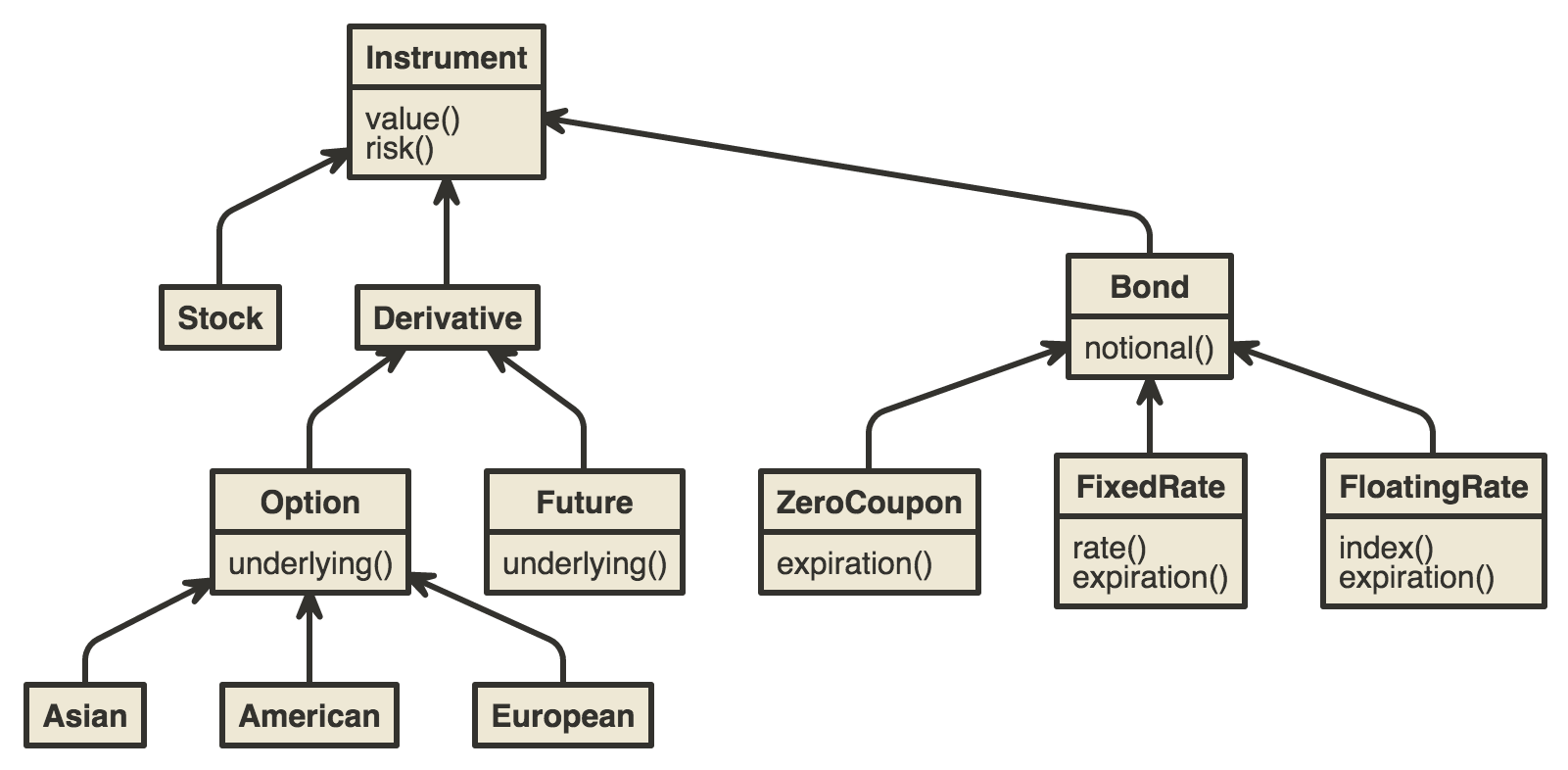
However, what happens if we want to add custom contracts?
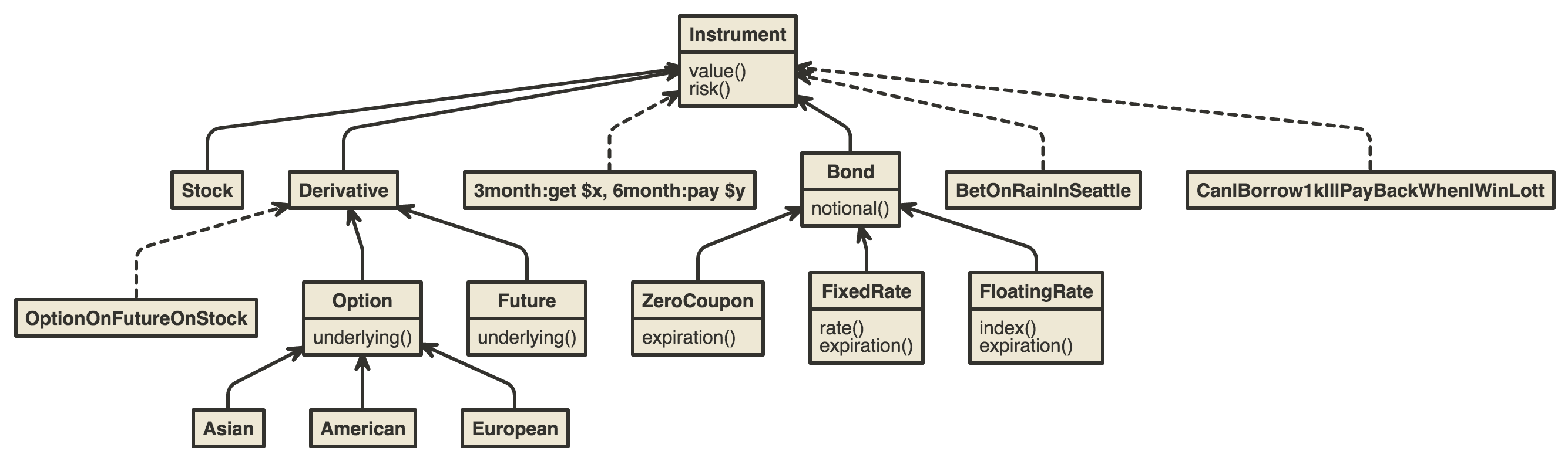
Notice that the root Instrument object contains a ‘value’ method, which returns its current value. In most cases, each class will implement it’s own valuation function. If, tomorrow, we discover a generalization, say Bond and another set of instruments can nicely fit under ‘Fixed Income’ class, we will either be forced to break the existing hierarchy or ignore the new generalization.
The combinator way
Peyton-Jones and Eber propose a completely different way of describing these contracts. They break up existing contracts into smaller components to find much more general and expressive pieces. When combined, not only do these smaller units describe existing contracts, but they are surprisingly effective at describing many custom and ad-hoc contracts.
Here are some examples:
def usd(amount) = Scale(Const(amount),One("USD"))
def stock(symbol) = Scale(Lookup(symbol),One("USD"))
def buy(contract, amount) = And(contract,Give(usd(amount)))
def sell(contract, amount) = And(Give(contract),usd(amount))
def zcb(maturity, notional, currency) = When(maturity, Scale(Const(notional),One(currency)))
def option(contract) = Or(contract,Zero())
def europeanCallOption(at, c1, strike) = When(at, option(buy(c1,strike)))
def europeanPutOption(at, c1, strike) = When(at, option(sell(c1,strike)))
def americanCallOption(at, c1, strike) = Anytime(at, option(buy(c1,strike)))
def americanPutOption(at, c1, strike) = Anytime(at, option(sell(c1,strike)))

val msft = stock("MSFT")
The paper describes a new language, made up of two types of combinators: contracts and observables. These combinators can be combined, as shown above, to describe instruments in one line, what may have taken days, weeks or even months to implement using typical methods.
Implementation
Let’s start with ‘Contract’ described below:
Contract is
  Zero -- This contract is worth $0.00
  or One -- $1.00
  or Give(Contract) -- -1 * value of Contract (rights of parties are reversed, lender becomes a borrower)
  or And(Contract,Contract) -- Combine values of both contracts
  or Or(Contract,Contract) -- Maximum of two contracts (we are assuming a rational person will always want more money)
  or Cond(Observable,Contract,Contract) -- standard 'if' statement
  or Scale(Observbale,Contract) -- Multiply value of Contract by Observable
  or When(Date,Contract) -- On Date, value is Contract, else $0.0
  or Anytime(Date,Contract) -- From now until Date, value is Contract, else $0.0
If you hold contract One, you are owed a dollar immediately (currency implications are ignored in this explanation, although not in the implementation). If you own Give(One()), you owe someone a dollar right away (not a few days from now). If you own When(tomorrow,One()), tomorrow someone will deposit a dollar in your account. If you own Anytime(next week, One()), you have the right to ask for your dollar anytime, between now and next week.
To make this even simpler, notice how many of the combinators can be mapped to basic math. Zero and One are simple enough. Give is just negation, And is addition, Or is Math.max(), Cond is ‘if … else …’ and Scale is multiplication of sorts. When and Anytime are only non-mathy items.
Note that I haven’t implemented the Until operator and When and Anytime take explicit dates, rather than the more generic Observable[Boolean] in the referenced paper.
Scale requires further comment, since it takes an Observable as an argument, not just Contract. Much of finance deals with future events. Stocks goes up, interest rates drop, a butterfly in China flaps wings and corn prices drop in Latin America. The language described by Contract alone is not able to represent real-world events. Since real-world events are uncertain, we need a way to represent this uncertainty. The Observable type manages this uncertainty for us. We can write contracts which depend on the price of Google’s stock, a year from now: When(next year, Scale(GOOG price, One())), and let Observable handle the details.
Observable is
  Const(c) -- Always returns c
  or Date() -- Always returns the date passed into observable
  or Lift1()
  or Lift2()
  or Lookup() -- Looks up real-world values
  or various math operators
Observables represent uncertain values across time. Think of an Observable as a function which takes a date, and returns a range of possible values. For example, if you want to represent the price of GOOG six months from now, Observable will do that for you. For the mathematically inclined, an Observable is a stochastic process. For a given date, it will return a random variable.
Const(10) will always return 10, no matter what the date. Date() will simply return the date you pass in to it. Lookup(“MSFT”) will return Microsoft’s future prices. Note that Lookup is not in the original papers, I added it so I could play around with equity derivatives.
Note that observables don’t actually implement any logic. They form a high level language (along with contracts), which is translated into a lower level implementation language.
LiftX functions may be confusing to non-functional programmers. Say, for whatever reason, you want to write a contract which takes square root of MSFT prices. You will notice that there is no square root combinator in Observable. Lift2(+) will ‘overload’ the plus function so it will also operate on Observable values.
Just for completeness, let’s paste the actual scala code here:
Scala definition of Contract and Obs(servable)
package ComposingContracts {

  sealed trait Contract
  case class Zero() extends Contract
  case class One(currency: String) extends Contract
  case class Give(contract: Contract) extends Contract
  case class And(contract1: Contract, contract2: Contract) extends Contract
  case class Or(contract1: Contract, contract2: Contract) extends Contract
  case class Cond(cond: Obs[Boolean], contract1: Contract, contract2: Contract) extends Contract
  case class Scale(scale: Obs[Double], contract: Contract) extends Contract
  case class When(date: LocalDate, contract: Contract) extends Contract
  case class Anytime(date: LocalDate, contract: Contract) extends Contract

  abstract class Obs[A] {
    def +(that: Obs[A])(implicit n: Numeric[A]): Obs[A] = Lift2(n.plus, this, that)
    def -(that: Obs[A])(implicit n: Numeric[A]): Obs[A] = Lift2(n.minus, this, that)
    ...
  }
  case class Const[A](k: A) extends Obs[A]
  case class Lift[B, A](lifted: (B) => A, o: Obs[B]) extends Obs[A]
  case class Lift2[C, B, A](lifted: (C, B) => A, o1: Obs[C], o2: Obs[B]) extends Obs[A]
  case class DateObs() extends Obs[LocalDate]
  case class Lookup[A](lookup: String) extends Obs[Double]
}
I’ll buy a One
Contracts and observables are all the end user sees. This domain specific language is enough to describe a large number of existing financial contracts, standardized as well us bespoke (or so the paper claims, assuming my own simplifications or errors didn’t render this useless). Note that the claim is NOT that this language will describe ALL financial contracts. For example, [“Certified Symbolic Management of Financial Contracts”] (http://www.pa-ba.net/pubs/entries/bahr14nwpt.html) by Bahr, Berthold and Elsman extends this language with an accumulator combinator to allow pricing of Asian options.
What about computation?
I have talked a lot about representing contracts. As Peyton-Jones and Eber point out, this, by itself, is quite remarkable. Such a descriptive language can be used to communicate effectively among companies, clients and regulators. However, what are the actual mechanics of pricing these contracts?
Before we get any further in the actual computation, let’s emphasize one point. The language which represents our universe of contracts has already been described. Nothing in the rest of this post will extend or modify that language. We now start the process of implementing the machinery which will price these contracts. Not only will the constructs of this machinery be invisible to end-users, we can swap out the existing implementation with a completely different mathematical model.
As the paper mentions, there are several popular ways of pricing financial contracts, including the lattice model, monte-carlo and finite differences. I have only implemented the lattice model. I chose this, in part because the paper itself describes it in greater detail than the other two methods, and because I was able to understand this method better than other models (remember, I have no training in financial engineering).
What’s it worth?
Before we get to the code, let’s delve a bit deeper into a fundamental concept, how to find a fair price for financial contracts. Wall Street employs so many people with math and science backgrounds that they have their own name: quants. People have won nobel prizes and earned billions of dollars by answering the question of pricing these contracts. Naturally, we will discuss only the most basic concepts.
A dollar today is worth more than a dollar tomorrow
How much are a thousand dollars worth? A thousand dollars! How much are a thousand dollars worth a year from now? The answer to this question involves [present discounted value] (http://en.wikipedia.org/wiki/Present_value). Let’s look for an intuitive explanation.
If you lend someone a thousand dollars for a year, how much should you get back? It would be silly if the borrower gave you $990 back. That’s ten dollars of hard cash less than you gave them. If they return your thousand dollars exactly, you are still losing money! If you hadn’t lent this money, you could have put it in your savings account and earned some (almost) guaranteed interest! So you should expect back your thousand dollars, plus the (almost) guaranteed interest rate you would have received. By the way, if you lent them money for two years, situation becomes slightly more complex. In two years, you can earn interest on your thousand dollars and in the second year, you can also earn interest on first year’s interest! Let’s leave any more detail and actual math behind discounting to the experts.
The basic idea is this, in order to know how much a future dollar is worth today, you need to know how far away that future is, and interest rates during that time.
Future’s uncertain
We can not predict the future, but can build models which take uncertainty into account. For this post, we will use a simple model of future prices.
Given today’s price, tomorrow’s price will either rise or drop proportional to volatility.
If an interest rate or a stock is S dollars today and historically it has moved up by ‘u’ or down by ‘d’, tomorrow it will be uS or dS, the day after it will be u^2S, d^2S or udS and so on. Why only two prices for tomorrow, instead of three or 8? Because this is the binomial lattice method, not trinomial or octonomial lattice method. Those who already know this method should note that we are ignoring probabilities here.

If you ask this data structure for today’s price, it will give you a single value, since that is already known. If you ask for any future dates, it will give you a range of values. In this specific model, day two will give you two values, day 10 will give you 10 values. The data structure is generally implemented as an list of arrays. If the whole lattice just contains a single number, we don’t bother using arrays and just return that constant. A few more such optimizations are made.
Note that with the popularization of machine learning, probabilistic programming, of which this is an example, has become a hot topic. This is an extremely interesting subject, so much so that I recently enrolled in a Master’s degree program at U Of Chicago to study this stuff. However, the existing implementation not not very elegant, general…or even completely correct.
Scala definition of the binomial lattice framework
trait BinomialLattice[A]{
  //apply functions allows this object to be 'called' as if it was a function
  def apply(i:Int):RandomVariable[A]
  //convenience 'apply' method allows use to think in terms of days, rather than just a integer index
  def apply(date:LocalDate):RandomVariable[A] = apply(ChronoUnit.DAYS.between(LocalDate.now(),date).toInt)
  def zip[B]...
  def map[B]...
  ...
}
//Actualy lattice structure needs to be bounded, otherwise implementation becomes very complex
trait BinomialLatticeBounded[A] extends BinomialLattice[A]{
  def size():Int
  ...
}
//If a value remains same, we can save memory by using ConstantBL
class ConstantBL[A](k:A) extends BinomialLattice[A]{
  override def apply(i:Int) = (j:Int)=>k
}
//Not quite ConstantBL, but deterministic
class PassThroughBL[A](func:(LocalDate)=>RandomVariable[A]) extends BinomialLattice[A]{
  override def apply(i:Int) = apply(LocalDate.now().plusDays(i))
  override def apply(i:LocalDate) = func(i)
}
class PassThroughBoundedBL[A](func:(LocalDate)=>RandomVariable[A], _size:Int) extends PassThroughBL[A](func) with BinomialLatticeBounded[A]{
  override def size() = _size
}
//Given a starting price and an up factor, generate the whole lattice
//NOTE: volatility is translated to up/down factor using a standard formula
class GenerateBL(_size:Int, startVal:Double, upFactor:Double, upProbability:Double=0.5) extends BinomialLatticeBounded[Double]{
  val cache = new ListBuffer[Array[Double]]
  val downFactor:Double = 1.0/upFactor

  cache.insert(0,Array(startVal))
  for(i <- 1 to size()-1){
    val arr = new Array[Double](i+1)
    arr(0) = downFactor * cache(i-1)(0)
    for(j <- 1 to i){
      arr(j) = upFactor * cache(i-1)(j-1)
    }
    cache.insert(i,arr)
  }
  override def apply(i:Int) = cache(i)
  override def size() = _size
}

//Given values of a lattice at the final date, apply function backwards towards start date
//Think of a discounting function, which takes future prices and uses interest rates to calculate current value
class PropagateLeftBL[A:ClassTag](source:BinomialLatticeBounded[A], func:((A,A)=>A)) extends BinomialLatticeBounded[A]{
  val cache = new ListBuffer[Array[A]]

  for(i <- 0 to size-1) cache.insert(i, new Array[A](i+1))

  for(i <- (0 to size-1).reverse){
    for(j <- (0 to i)){
      val x = source(i+1)(j)
      val y = source(i+1)(j+1)
      cache(i)(j) = func(x,y)
    }
  }

  override def apply(i:Int) = if ( size() > 1) cache(i) else source(i)
  override def size() = if (source.size() > 1) source.size()-1 else 1
}
A couple of supporting functions. binomialPriceTree takes a starting price, date range and volatility and converts it to a binomial lattice. Note this is very similar to the GenerateBL class. The only difference here is that binomailPriceTree converts volatility ot up/down factors. dicount method takes two lattices, one contains the data which needs to be discounted and the second contains the interest rates which will be used to do the discounting.
def binomialPriceTree(days:Int, startVal:Double, annualizedVolatility:Double, probability:Double=0.5):BinomialLatticeBounded[Double] = {

  val businessDaysInYear = 365.0
  val fractionOfYear = (days* 1.0) divide businessDaysInYear
  val changeFactorUp = vol2chfactor(annualizedVolatility,fractionOfYear)
  val process = new GenerateBL(days+1,startVal,changeFactorUp)
  process
}

def vol2chfactor(vol:Double, fractionOfYear:Double) = {
  Math.exp(vol * Math.sqrt(fractionOfYear))
}

def discount(toDiscount:BinomialLatticeBounded[Double], interestRates:BinomialLattice[Double]):BinomialLatticeBounded[Double] = {
  val averaged = new PropagateLeftBL[Double](toDiscount, (x,y)=>(x+y) divide 2.0)//assume .5 probability
  val zipped = averaged.zip(interestRates)
  zipped.map[Double](avg_ir=>{
    val avg = avg_ir._1
    val ir = avg_ir._2
    avg/(1.0+ir)
    })
}
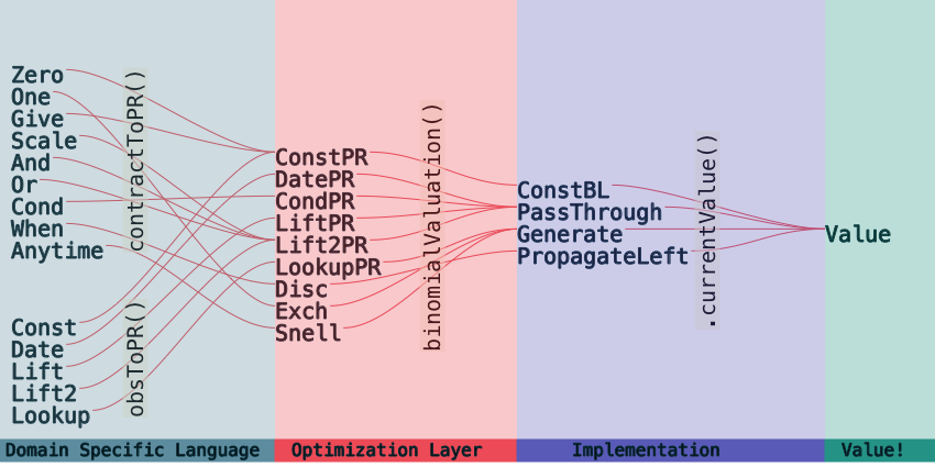
Tie them together
We have seen the contract description language and some gory details of how a binomial lattice is implemented. We don’t yet have a path connecting the two. Contract and Observable, both, are translated to a lower level abstract layer called PROpt, meaning “process optimization layer.” A process, as mentioned earlier, represents a time varying value. Given a date, a process returns a random variable. BinomialLattice implements this, but PROpt is a layer between Contract/Observable and BinomialLattice.
The paper shows how to use this layer to do some optimizations. Unfortunately I ran out of time and didn’t implement that code when this post was written.
Scala definition of optimization layer
abstract class PROpt[A] {
...
}
case class ConstPR[A]       (k: A)                                            extends PROpt[A]
case class DatePR           ()                                                extends PROpt[LocalDate]
case class CondPR[A]        (cond: PROpt[Boolean], a: PROpt[A], b: PROpt[A])  extends PROpt[A]
case class LiftPR[B, A]     (lifted: (B) => A, o: PROpt[B])                   extends PROpt[A]
case class Lift2PR[C, B, A] (lifted: (C, B) => A, o1: PROpt[C], o2: PROpt[B]) extends PROpt[A]
case class LookupPR[A]      (lookup:String)                                   extends PROpt[Double]

case class Snell[A]         (date:LocalDate, c: PROpt[Double])                extends PROpt[Double]
case class Disc[A]          (date:LocalDate, c: PROpt[Double])                extends PROpt[Double]
case class Absorb[A]        (date:LocalDate, c: PROpt[Double])                extends PROpt[Double]
case class Exch[A]          (curr: String)                                    extends PROpt[Double]
How contracts and observables are mapped to combinators of the optimization layer. Note that the code below is essentially mapping objects form higher level language to lower level language. For example:
Zero() => ConstPR(0)
This just means that Zero, from Contract, translates to ConstPR(0) in PROpt. Function contractToPROpt maps contracts to PROpt while obsTOPROpt maps observables.
def contractToPROpt(contract: Contract): PROpt[Double] = contract match {
  case Zero()                                => ConstPR(0)
  case One(currency)                         => Exch(currency)
  case Give(c: Contract)                     => contractToPROpt(Scale(Const(-1), c))
  case Scale(o: Obs[Double], c: Contract)    => Lift2PR((a: Double, b: Double) => a * b, obsToPROpt(o), contractToPROpt(c))
  case And(c1: Contract, c2: Contract)       => Lift2PR((a: Double, b: Double) => a + b, contractToPROpt(c1), contractToPROpt(c2))
  case Or(c1: Contract, c2: Contract)        => Lift2PR((a: Double, b: Double) => Math.max(a, b), contractToPROpt(c1), contractToPROpt(c2))
  case Cond(o: Obs[Boolean], c1: Contract, c2: Contract) => CondPR(obsToPROpt(o), contractToPROpt(c1), contractToPROpt(c2))
  case When(date: LocalDate, c: Contract)    => Disc(date, contractToPROpt(c))
  case Anytime(date: LocalDate, c: Contract) => Snell(date, contractToPROpt(c))
}

def obsToPROpt[A](observable: Obs[A]): PROpt[A] = observable match {
  case Const(k)              => ConstPR(k)
  case Lift(func, o: Obs[A]) => LiftPR(func, obsToPROpt(o))
  case Lift2(func, o1, o2)   => Lift2PR(func, obsToPROpt(o1), obsToPROpt(o2))
  case DateObs()             => DatePR()
  case Lookup(lookup)        => LookupPR(lookup)
}
Note that the PROpt layer exists as a non-implementation level layer which can be used to do some optimizations. We don’t do any optimizations here so it might seem unnecessary.
Translate optimization layer to binomial lattice
Similar to how we translated contracts and observables to PROpt, the following code translates PROpt to BinomialLattice, defined earlier.
Notice that binomialValuation method takes an argument of type Environment. This environment, or ‘context,’ as some frameworks might call it, contains much of our real-world information. This contains actual interest rates, currency exchange rates, volatility, etc.
def binomialValuation[A](pr: PROpt[A], marketData: Environment): BinomialLattice[A] = pr match {
  case ConstPR(k) => new ConstantBL(k)
  case DatePR() => new PassThroughBL((date:LocalDate)=>(idx:Int)=>date)
  case CondPR(cond: PROpt[Boolean], a: PROpt[A], b: PROpt[A]) => {
    val o = binomialValuation(cond, marketData)
    val ca = binomialValuation(a, marketData)
    val cb = binomialValuation(b, marketData)

    new PassThroughBL[A](
      (date: LocalDate) => (idx: Int) => if (o(date)(idx)) ca(date)(idx) else cb(date)(idx)
      )
  }
  case LiftPR(lifted, o) => {
    val obs = binomialValuation(o, marketData)
    new PassThroughBL[A](
      (date: LocalDate) => (idx: Int) => lifted(obs(date)(idx))
      )
    }
    case Lift2PR(lifted, o1, o2) => {
      val obs1 = binomialValuation(o1, marketData)
      val obs2 = binomialValuation(o2, marketData)
      new PassThroughBL[A](
        (date: LocalDate) => (idx: Int) => lifted(obs1(date)(idx), obs2(date)(idx))
        )
    }
    case LookupPR(lookup) => {
      marketData.lookup(lookup)
    }
    case Exch(curr: String) => {
      val exchangeRate = marketData.exchangeRates(curr)
      new PassThroughBL[A](
        (date: LocalDate) => (idx: Int) => exchangeRate(date)(idx)
        )
    }
    case Disc(date: LocalDate, c: PROpt[Double]) => {
      val daysUntilMaturity = ChronoUnit.DAYS.between(LocalDate.now(), date).toInt
      val con = binomialValuation(c, marketData)
      val interestRates = marketData.interestRate

      val _process = new PassThroughBoundedBL[Double]((date:LocalDate)=>(idx:Int)=>con(date)(idx),daysUntilMaturity+1)//daysUntilMaturity+1 because if contract matures today, it still needs today's valuation
      discount(_process,interestRates)
    }
    case Snell(date: LocalDate, c: PROpt[Double]) => {
      /*
      Take final column of the tree, discount it back one step. Take max of the discounted column and the original column, repeat.
      */
      val daysUntilMaturity = ChronoUnit.DAYS.between(LocalDate.now(), date).toInt
      val con = binomialValuation(c, marketData)
      val interestRates = marketData.interestRate

      val _process:BinomialLatticeBounded[Double] = new PassThroughBoundedBL[Double]((date:LocalDate)=>(idx:Int)=>con(date)(idx),daysUntilMaturity+1)//daysUntilMaturity+1 because if contract matures today, it still needs today's valuation
      var result = _process
      for(i <- 0 to _process.size()){
        val discounted:BinomialLatticeBounded[Double] = discount(result,interestRates)
        val contractAndDiscounted:BinomialLatticeBounded[(Double,Double)] = discounted.zip(_process)
        result = contractAndDiscounted.map[Double]((cNd)=>{
          val c = cNd._1
          val d = cNd._2
          Math.max(c,d)
        })
      }
      result
    }
  }
Run a test
Scala’s equivalent of the ‘main’ method. This code keeps us honest, since it actually exercises the api/language we have developed.
object Main extends App {
  //Required for doing LocalDate comparisons...a scalaism
  implicit val LocalDateOrdering = scala.math.Ordering.fromLessThan[java.time.LocalDate]{case (a,b) => (a compareTo b) < 0}

  //custom contract
  def usd(amount:Double) = Scale(Const(amount),One("USD"))
  def buy(contract:Contract, amount:Double) = And(contract,Give(usd(amount)))
  def sell(contract:Contract, amount:Double) = And(Give(contract),usd(amount))
  def zcb(maturity:LocalDate, notional:Double, currency:String) = When(maturity, Scale(Const(notional),One(currency)))
  def option(contract:Contract) = Or(contract,Zero())
  def europeanCallOption(at:LocalDate, c1:Contract, strike:Double) = When(at, option(buy(c1,strike)))
  def europeanPutOption(at:LocalDate, c1:Contract, strike:Double) = When(at, option(sell(c1,strike)))
  def americanCallOption(at:LocalDate, c1:Contract, strike:Double) = Anytime(at, option(buy(c1,strike)))
  def americanPutOption(at:LocalDate, c1:Contract, strike:Double) = Anytime(at, option(sell(c1,strike)))

  //custom observable
  def stock(symbol:String) = Scale(Lookup(symbol),One("USD"))
  val msft = stock("MSFT")


  //Tests
  val exchangeRates = collection.mutable.Map(
    "USD" -> LatticeImplementation.binomialPriceTree(365,1,0),
    "GBP" -> LatticeImplementation.binomialPriceTree(365,1.55,.0467),
    "EUR" -> LatticeImplementation.binomialPriceTree(365,1.21,.0515)
    )
  val lookup = collection.mutable.Map(
    "MSFT" -> LatticeImplementation.binomialPriceTree(365,45.48,.220),
    "ORCL" -> LatticeImplementation.binomialPriceTree(365,42.63,.1048),
    "EBAY" -> LatticeImplementation.binomialPriceTree(365,53.01,.205)
  )
  val marketData = Environment(
    LatticeImplementation.binomialPriceTree(365,.15,.05), //interest rate (use a universal rate for now)
    exchangeRates, //exchange rates
    lookup
  )

  //portfolio test
  val portfolio = Array(
    One("USD")
    ,stock("MSFT")
    ,buy(stock("MSFT"),45)
    ,option(buy(stock("MSFT"),45))
    ,americanCallOption(LocalDate.now().plusDays(5),stock("MSFT"),45)
  )

  for(contract <- portfolio){
    println("===========")
    val propt = LatticeImplementation.contractToPROpt(contract)
    val rp = LatticeImplementation.binomialValuation(propt, marketData)
    println("Contract: "+contract)
    println("Random Process(for optimization): "+propt)
    println("Present val: "+rp.startVal())
    println("Random Process: \n"+rp)
  }

}
Full code is available at https://github.com/falconair/ComposingContracts
Take a step back
Let’s get an overview of what we’ve actually done
We started with a high level language to describe financial contracts. This was represented by Contract and Obs(servable) combinators. These were essentially empty classes with no implementation.
Contracts and observables were translated to a single set of combinators in the optimization layer. After optimization (which we never did), we translated to the actual implementation layer, which contains code to actually price these instruments.
Work left undone
As mentioned earlier, the paper shows how to do some basic optimizations. For example, Give(Give(One(“USD”))) is the same as One(“USD”) and exchange rate of USD to USD is constant. As I write this, I have not implemented these optimizations. As I also mentioned earlier, I also didn’t implement the Until contract combinator, and consequently, the Absorb combinator in the optimization layer. In order to get this post out in time, I decided to leave some features aside.
Future direction
If I ever get back to this code, I’ll be particularly interested in exploring some interesting ideas not mentioned in the paper.
I mentioned earlier that Contract combinators seem to correspond roughly to basic operator from algebra. Zero, One, +, *, negate, etc. I have no training in abstract math so I don’t know if this dsl actually forms an interesting structure from mathematics. However, if it does, what might that mean? I’m reminded of correspondence between computer science type theory and algebra. For example, [this] (http://chris-taylor.github.io/blog/2013/02/10/the-algebra-of-algebraic-data-types/) post by Chris Taylor (and the linked YouTube talk) shows how data types can be thought of as a kind of algebra, complete with equations the ability to do calculus! Thinking of types at the level of algebra leads to interesting benefits such as discovery of the zipper data structure. What might it mean to solve for an unknown variable in the language we have developed here? What might it mean to do calculus on expressions of this language?
The paper mentions that this language uses some concepts from Conal Elliott’s [Fran] (http://conal.net/fran/) language. Fran was one of the first languages to introduce (or popularize) Functional Reactive Programming. In recent years, FRP’s semantics have been described using temporal logic, using operators ‘always’ and ‘eventually.’ Unfortunately even the abstracts of these papers make no sense to me. However, Could When and Anytime be re-written in terms of ‘always’ and ‘eventually’ from temporal logic? The language introduced in composing contracts is so interesting because someone took the time to break apart conventional thinking about financial instruments and put the pieces back together in an, arguably, more expressive and elegant manner. What if there are yet more expressive and general combinators? [This] (http://www.ioc.ee/~wolfgang/research/plpv-2013-paper.pdf) paper by Wolfgang Jeltsch might provide a hint. The paper shows how ‘always’ and ‘eventually,’ used in semantics of FRP can be generalized further with an ‘until’ operator! At least what I think the paper is saying.
Closer to my skills, how else could this language be used? Couldn’t we build a ‘universal’ exchange, which knows how to trade any financial instrument and even correlated products? Couldn’t this language be used to automatically figure out correct hedges, even for complex portfolios? Since this language describes contracts in a declarative manner, couldn’t we use something like genetic programming to evolve ever more profitable contracts? About that…
“Beware of geeks bearing formulas” - Warren Buffet
The 2007-2008 market crash was blamed, in large part, on financial contracts so complex that no one really understood their consequences. These contracts and the mathematical models behind them, made assumptions that just didn’t hold. Countless people lived in misery for years, many still do. A misunderstood assumption in the financial markets can cause real-world pain. Be careful with this stuff.
Some notes on the paper
I read somewhere that Jean-Marc Eber had been thinking financial instruments being composable for ten years, before he co-wrote the first version of the paper. Coming up with smaller, more composable and more elegant combinators doesn’t seem to be easy! However, benefits are immense!
Since this paper was published, others have extended this language so it can describe more general commercial contracts, such as rental agreements(1) or lawyer services! [Work] (http://www.diku.dk/~paba/pubs/files/bahr14nwpt-extended%20abstract.pdf)(2) has been done to formalize the language further and having an automated proof checker confirm that contracts make sense. Since some pricing methods, such as monte carlo improve accuracy of prices at a huge computational cost, an attempt has been made to automatically [map] (http://hiperfit.dk/pdf/WerkAhnfelt_2011-10ab.pdf)(3) computation to GPUs has been written. Unfortunately I’ve lost references to several interesting papers which extend this work.
Gratitude
Writing code for this paper was very enjoyable indeed. In the process I kicked the tires a bit more on Scala and came away impressed. The whole implementation comes in at less than 500 lines.
I want to thank Simon Peyton-Jones and Jean-Marc Eber, not only for writing this awesome paper, but also for answering my questions! Mr. Eber, who must be very busy running a successful company, Lexifi, based on the principles outlined in this paper, actually replied to my queries in a very thoughtful and generous manner.
Soon after I first read this paper, I was lucky enough to attend Anton Van Straaten’s talk on the topic in New York City. Although his code no longer seems to be available, his Haskell implementation was short and beautiful (from what I recall, he even used a charting package to show how these instruments’ prices change). I obviously don’t remember much from that presentation anymore, but his talk gave me confidence that this stuff was actually implementable.
This being my second project in Scala, tpolecat, Kristien and OlegYch on #scala chat room on freenode helped me immensely. If it wasn’t for their help, I would have struggled for weeks to solve scala related problems.
Finally, thanks to my colleague Amit Pandey for helping me understand the Snell operator.
- Binomial lattice from http://stackoverflow.com/a/20911612/46799
- [Compositional specification of commercial contracts] (http://www.itu.dk/~elsborg/sttt06.pdf) by Andersen, Elsborg, Henglein, Simonsen and Stefansen
- [Towards Certified Management of Financial Contracts] (http://www.diku.dk/~paba/pubs/files/bahr14nwpt-extended%20abstract.pdf) by Bahr, Berthold and Elsman
- [Pricing composable contracts on the GP-GPU] (http://hiperfit.dk/pdf/WerkAhnfelt_2011-10ab.pdf) by Ahnfelt-Ronne and Werk.
Let me know!
Checkout http://forum.targetcompid.com. A community site by and for trading technologists.